Input data structure¶

The input data is structured in a folder hierarchy. The root folder <data_folder> contains a subfolder for each dataset and a configuration file config.json. ZEN-garden is run from this root folder (Running a model). The dataset folder <dataset> comprises the input data for a specific dataset and must contain the following files and subfolders:

<data_folder>/
|--<dataset>/
|   |--energy_system/
|   |   |--attributes.json
|   |   |--base_units.csv
|   |   |--set_nodes.csv
|   |   `--set_edges.csv
|   |
|   |--set_carriers/
|   |   |--<carrier1>/
|   |   |   `--attributes.json
|   |   `--<carrier2>/
|   |       `--attributes.json
|   |
|   |--set_technologies/
|   |   |--set_conversion_technologies/
|   |   |   |--<conversion_technology1>/
|   |   |   |   `--attributes.json
|   |   |   |
|   |   |   `--<conversion_technology2>/
|   |   |       `--attributes.json
|   |   |
|   |   |--set_storage_technologies/
|   |   |      `--<storage_technology1>/
|   |   |          `--attributes.json
|   |   |
|   |   `--set_transport_technologies/
|   |       `--<transport_technology1>/
|   |           `--attributes.json
|   |
|   `--system.json
|
`--config.json

Note that all folder names in <> in the structure above can be chosen freely. The dataset is described by the properties of the energy_system, the set_carriers, and the set_technologies. The system configuration is stored in the file system.json and defines dataset-specific settings, e.g., which technologies to model or how many years and time steps to include. The configuration file config.json contains more general settings for the optimization problem and the solver. Refer to the section Configurations for more details.

Depending on your analysis, more files can be added; see Attribute.json files and Tutorial 4: Create Scenarios for more information.

Folders¶

Energy System¶

The folder energy_system contains four necessary files: attributes.json, base_units.csv, set_nodes.csv, and set_edges.csv. The file attributes.json defines the numerical setup of the energy system, e.g., the carbon emission limits, the discount rate, or the carbon price. set_nodes.csv and set_edges.csv define the nodes and edges of the energy system graph, respectively. set_nodes.csv contains the coordinates of the nodes, which are used to calculate the default distance of the edges.

There is no predefined convention for naming nodes and edges, so the user can choose the naming freely. In the examples, we use <node1>-<node2> to name edges, but note that you are not forced to follow that convention. In fact, set_edges.csv defines the edges by the nodes they connect.

Note

You can specify more nodes in set_nodes.csv than you end up using. In system.json you can define a subset of nodes you want to select in the model. If you do not specify any nodes in system.json, all nodes from set_nodes.csv are used.

base_units.csv define the base units in the model. That means that all units in the model are converted to a combination of base units. See Tutorial 6: Unit consistency for more information.

Technologies¶

The set_technologies folder is specified in three subfolders: set_conversion_technologies, set_storage_technologies, and set_transport_technologies. Each technology has its own folder in the respective subfolder and must contain the attributes.json file. Additional files can further parametrize the technologies (see Attribute.json files).

Note

You can specify more technologies in the three subfolders than you end up using. That can be helpful if you want to model different scenarios with different technologies and carriers.

Each technology has a reference carrier, i.e., that carrier by which the capacity of the technology is rated. As an example, a \(10kW\) heat pump could refer to \(10kW_{th}\) heat output or \(10kW_{el}\) electricity input. Hence, the user has to specify which carrier is the reference carrier in the file attributes.json. For storage technologies and transport technologies, the reference carrier is the carrier that is stored or transported, respectively.

Conversion Technologies¶

The conversion technologies are defined in the folder set_conversion_technologies. A conversion technology converts 0 to n input carriers into 0 to m output carriers. Note that the conversion factor between the carriers is fixed, e.g., a combined heat and power (CHP) plant cannot sometimes generate more heat and sometimes generate more electricity. The file attributes.json defines the properties of the conversion technology, e.g., the capacity limit, the maximum load, the conversion factor, or the investment cost.

A special case of the conversion technologies are retrofitting technologies. These technologies are defined in the folder set_conversion_technologies\set_retrofitting_technologies, if any exist. They behave equal to conversion technologies, but they are always connected to a conversion technology. They are coupled to a conversion technology by the attribute retrofit_flow_coupling_factor in the file attributes.json, which couples the reference carrier flow of the retrofitting technology and the base technology. A possible application of retrofitting technologies is the installation of a carbon-capture unit on top of a power plant. In this case, the base technology would be power_plant and the retrofitting technology would be carbon_capture. Refer to the dataset example 14_retrofitting_and_fuel_substitution for more information.

Storage Technologies¶

The storage technologies are defined in the folder set_storage_technologies. A storage technology connects two time steps by charging at t=t0 and discharging at t=t1.

Note

In ZEN-garden, the power-rated (charging-discharging) capacity and energy-rated (storage level) capacity of storage technologies are optimized independently. If you want to fix the energy-to-power ratio, the attribute energy_to_power_ratio in attributes.json can be set to anything different than inf.

Transport Technologies¶

The transport technologies are defined in the folder set_transport_technologies. A transport technology connects two nodes via an edge. Different to conversion technologies or storage technologies, transport technology capacities are built on the edges, not the nodes.

Note

By default, the distance of an edge will be calculated as the haversine distance between the nodes. This can be overwritten for specific edges in a distance.csv file (see Attribute.json files).

Carriers¶

Each energy carrier is defined in its own folder in set_carriers. You do not need to specify the used energy carriers explicitly in system.json, but the carriers are implied from the used technologies. All input, output, and reference carriers that are used in the selected technologies (see input_structure.technologies) must be defined in the set_carriers folder. The file attributes.json defines the properties of the carrier, e.g., the carbon intensity or the cost of the carrier. Additional files can further parametrize the carriers (see Attribute.json files).

Note

You can specify more carriers in set_carriers than you end up using. That can be helpful if you want to model different scenarios with different technologies and carriers.

Files¶

Attribute.json files¶

Each element in the input data folder has an attributes.json file, as shown in Input data structure, which defines the default values for the element. This file must be specified for each element and must contain all parameters that this class of elements (Technology, Carrier, etc.) can have (see Notation: Sets, parameters, variables, and constraints).

The attributes.json files have three main purposes:

Defining all parameters of each element
Providing the default value for each parameter
Defining the unit of each parameter

How are `attributes.json` files structured?¶

The general structure of each attributes.json file is the following:

{
  "parameter_1": {
    "default_value": v_1,
    "unit": "u_1"
  },
  "parameter_2": {
    "default_value": v_2,
    "unit": "u_2"
  },
  ...
}

The structure is a normal dictionary structure. Make sure to have the correct positioning of the brackets.

There is one curly bracket around all parameters {...}
Each parameter has a name, followed by a colon and curly brackets name: {...}
Inside the curly brackets are in most cases a default_value as a float or "inf" and a unit as a string (see Tutorial 6: Unit consistency).

Special parameters in the `attributes.json` file¶

Some technology parameters do not have the structure above. These are: "input_carrier", "output_carrier", "reference_carrier", "conversion_factor" (for conversion technologies only), and "retrofit_flow_coupling_factor" (for retrofitting technologies only).

Input, output, and reference carriers

The input and output carriers refer to the energy carriers which a technology takes as input or output. The data format for these attributes differs since technologies can have more than one input or output carrier. Consequentially, these attributes take a list [..., ...] rather than a single value such as "inf" or 0. The JSON below, for example, describes the Haber-Bosch process, which converts hydrogen and electricity to ammonia.

"reference_carrier": {
  "default_value": [
    "ammonia"
  ]
},
"input_carrier": {
  "default_value": [
    "hydrogen",
    "electricity"
  ]
},
"output_carrier": {
  "default_value": [
    "ammonia"
  ]
}

The reference_carrier attribute defines the carrier based on which technology performance is measured. It must be one of the input or output carriers. In the Haber-Bosch process describe above, for example, the reference carrier is ammonia. This means that the capacity of the Haber-Bosch facility is defined in terms of ammonia output per unit time (rather than e.g. the hydrogen consumed per unit time). It also means that the conversion factors for the technology (see below) must be defined relative to the ammonia output.

The following properties must hold for all carriers:

The reference carrier is one of the input or output carriers.
The input and output carriers must be mutually exclusive (i.e. no carrier can be both).
All carriers must be defined by attributes.json files within their respective folders set_carriers\<carrier_name>.

The units of the input, output, and reference carriers are defined by carrier parameters (see Tutorial 6: Unit consistency). They are therefore omitted in the "reference_carrier", "input_carrier", and "output_carrier" fields.

Conversion factor

The conversion_factor is the ratio between a carrier flow and the reference carrier flow. It is defined for all input carriers and output carriers that are not the reference carrier. The conversion factor sets the efficiency of a technology at converting between the input and output carriers. The units of the conversion factor are always <unit of carrier>/<unit of reference carrier>.

For the Haber-Bosch process, the conversion factor could for example be defined as:

"conversion_factor": [
  {
    "electricity": {
      "default_value": 0.05,
      "unit": "GW/GW"
    }
  },
  {
    "hydrogen": {
      "default_value": 0.95,
      "unit": "GW/GW"
    }
  }
]

This format consists of a list [...] in which each carrier (excluding the reference carrier) is wrapped in curly brackets. Inside each curly bracket, there are the default_value and the unit attributes. The above JSON means that the Haber-Bosch process consumes 0.05 GW of electricity and 0.95 GW of hydrogen per unit of ammonia produced. The conversion factors for the Haber-Bosch process are expressed per unit of ammonia since ammonia is defined as the reference carrier.

Retrofitting flow coupling factor

The retrofitting flow coupling factor couples the reference carrier flow of the retrofitting technology and the base technology (Conversion Technologies). The default value is defined in attributes.json as:

"retrofit_flow_coupling_factor": {
  "base_technology": <base_technology_name>,
  "default_value": 0.5,
  "unit": "GWh/GWh"
}

The retrofitting flow coupling factor is a single parameter with the base technology as a string and the default value and unit as usual.

Overwriting default values¶

The paradigm of ZEN-garden is that the user only has to specify those input data that they want to specify. Therefore, the user defines default values for all parameters in the attributes.json files. Whenever more information is required, the user can overwrite the default values by providing a <parameter_name>.csv file in the same folder as the attributes.json file.

Let’s assume the following example: The purpose of the energy system is to provide heat, whose default demand is given as 10 GW:

{
  "demand": {
    "default_value": 10,
    "unit": "GW"
  }
}

The energy system is modeled for two nodes, CH and DE and spans one year with 8760 time steps.

Note

To retrieve the dimensions of a parameter, please refer to Notation: Sets, parameters, variables, and constraints and to the index_names attribute in the parameter definition.

Providing extra .csv files¶

If the user wants to specify the demand CH and DE in the time steps 0, 14, 300, the user can create a file demand.csv:

node,time,demand
CH,0,5
CH,14,7
CH,300,3
DE,0,2
DE,14,3
DE,300,2

The file overwrites the default value for the demand at nodes CH and DE in time steps 0, 14,300.

Note

ZEN-garden will select that subset of data that is relevant for the optimization problem. If the user specifies a demand for a node in demand.csv that is not part of the optimization problem, the demand is ignored for this node.

To avoid overly long files, the dimensions can be unstacked, i.e., the values of one dimension can be the column names of the file:

node,0,14,300
CH,5,7,3
DE,2,3,2

time,CH,DE
0,5,2
14,7,3
300,3,2

Therefore, the full demand time series is 10 GW except for the time steps 0, 14, 300 where it is 5 GW, 7 GW, 3 GW for CH and 2 GW, 3 GW, 2 GW for DE.

Warning

Make sure that the unit of the values in the .csv file is consistent with the unit defined in the attributes.json file! Since we do not specify a unit in the .csv file, the unit of the values is assumed to be the same as the unit in the attributes.json file.

Constant dimensions¶

Often, we have parameters that are constant over a certain dimension but change with another dimension. For example, the demand of an industrial energy carrier might be constant over time but is different for all nodes.

In this case, the full demand.csv file would be:

node,0,1,2,...,8760
CH,5,5,5,...,5
DE,2,2,2,...,2

This is a very long file, and it is hard to see the structure of the data. Furthermore, it is prone to errors. Therefore, ZEN-garden allows you to drop dimensions that are constant. The file can be shortened to:

node,demand
CH,5
DE,2

The file is much shorter and easier to read. ZEN-garden will automatically fill in the missing dimensions with the constant value.

Yearly variation¶

We specify hourly-dependent data for each hour of the year. However, some parameters might have a yearly variation, e.g., the overall demand may increase or decrease over the years.

To this end, the user can specify a file <parameter_name>_yearly_variation.csv that multiplies the hourly-dependent data with a factor for each hour of the year. ZEN-garden therefore assumes the same time series for each year but allows for the scaling of the time series with the yearly variation. Per default, the yearly variation is assumed to be 1. Therefore, for missing values in <parameter_name>_yearly_variation.csv, the hourly-dependent data is not scaled.

Warning

The <parameter_name>_yearly_variation.csv only works for parameters which vary on an hourly basis. It therefore does not work for parameters such as capacity that only have one value per year. For such parameters, yearly variation must be specified directly in the <parameter_name>.csv file.

The user can specify the yearly variation for all dimensions except for the time dimension:

node,2020,2021,2022,...,2050
CH,1,1.1,1.2,...,4
DE,1,0.99,0.98,...,0.7

If all nodes have the same yearly variation, the file can be shortened to:

year,demand_yearly_variation
2020,1
2021,1.1
2022,1.2
...
2050,4

Note

So far, ZEN-garden does not allow for different time series for each year but only for the scaling while keeping the same shape of the time series.

Data interpolation¶

To reduce the number of data points, ZEN-garden per-default interpolates the data points linearly between the given data points. As an example, in Yearly variation, the demand increase or decrease is linear over the years. So, the user can reduce the number of data points in the demand_yearly_variation.csv file:

year,demand_yearly_variation
2020,1
2050,4

If the user wants to disable the interpolation for a specific parameter, the user can create a parameters_interpolation_off.json file and specify the parameter names in the file:

{
  "parameter_name": [
    "carbon_emissions_annual_limit",
    "demand_yearly_variation"
  ]
}

Note

The user must specify the file name, i.e., in the example above, the specified file is demand_yearly_variation.csv, not demand.csv. Therefore, the interpolation is only disabled for the yearly variation, not for the hourly-dependent data.

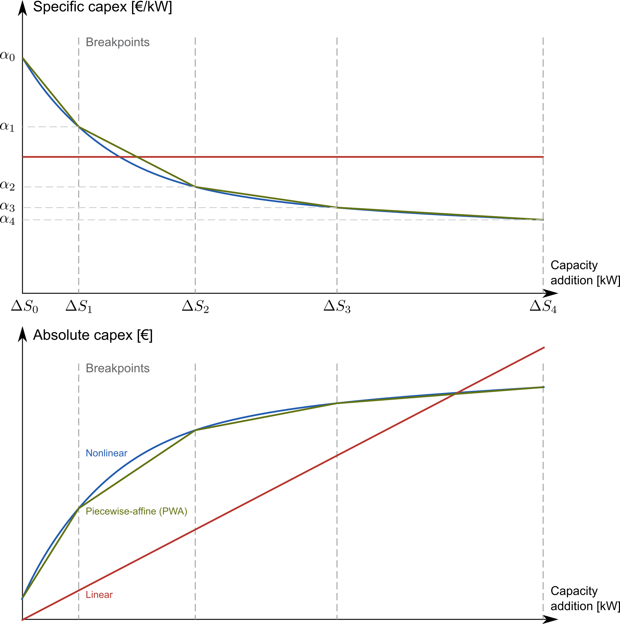
Piece-wise affine input data¶

In ZEN-garden, we can model the capital expenditure (CAPEX) of conversion technologies either linear or piece-wise affine (PWA). In the linear case, the capex_specific_conversion parameter is treated like every other parameter, i.e., the user can specify a constant value and a .csv file.

In the PWA case, the user can specify a nonlinear_capex.csv file that contains the breakpoints and the CAPEX values of the PWA representation. A PWA representation is a set of linear functions that are connected at the breakpoints. The breakpoints are the capacity additions \(\Delta S_m\) with the corresponding CAPEX values \(\alpha_m\).

Piece-wise affine representation of CAPEX

The file nonlinear_capex.csv has the following structure:

capacity_addition,capex_specific_conversion
0,2000
20,1700
40,1500
60,1350
80,1200
100,1100
120,1010
140,940
160,890
180,860
200,840
GW,Euro/kW

Note

Each new interval between two breakpoints adds a binary variable to the optimization problem, for each technology, each year, and each node. The binary variable is 1 if the capacity is in the interval and 0 otherwise. The user is advised to keep the number of breakpoints low to avoid a combinatorial explosion of binary variables.

Input data structure¶

Folders¶

Energy System¶

Technologies¶

Conversion Technologies¶

Storage Technologies¶

Transport Technologies¶

Carriers¶

Files¶

Attribute.json files¶

How are attributes.json files structured?¶

Special parameters in the attributes.json file¶

Overwriting default values¶

Providing extra .csv files¶

Constant dimensions¶

Yearly variation¶

Data interpolation¶

Piece-wise affine input data¶

How are `attributes.json` files structured?¶

Special parameters in the `attributes.json` file¶