Tutorial 1: Analyze Outputs
This tutorial describes how to analyze the the outputs of the ZEN-garden model. Two approaches are introduced:
The ZEN-garden visualization platform
The ZEN-garden
Resultsobject.
The visualization platform is an ideal starting point for data analysis. The platform allows user to see standardized plots of capacity mixes, generation mixes, energy balances, technology locations. The platform is interactive, allowing users to select what regions, time-steps, and scenarios, and energy carriers to view results from. In contrast, the results object is ideal for detailed analyses where users work directly with the model output and produce custom plots or calculations. The results object allows users to easily filter, extract, and compare results from various scenarios.
This tutorial assumes that you have installed and run the example dataset
5_multiple_time_steps_per_year as described in the tutorial setup
instructions. It also assumes that the ZEN-garden conda
environment is already activated (see instructions). The raw results of each ZEN-garden simulation are
stored in the following path relative to the data folder:
data\output\<dataset_name>.
Tip
The results are self-contained, i.e., you can copy the <dataset_name>
folder to another location and still access the results.
Visualization Platform
Running the Platform
Use the following steps to run the visualization platform:
In a terminal window, navigate to the
datafolder which contains the input data for the example model and the newly generatedoutputfolder.cd /path/to/your/data
Activate the ZEN-garden environment in case it is not already activated (see instructions). Then, run the following command:
zen-visualization
Running this command will pull up a new tab in your default browser containing the visualization platform. If the tab does not open automatically, you can open http://localhost:8000/ in any browser of your choice.
Tip
To exit the visualization tool, press Control + C in the terminal window.
Note
By default, the suite looks for solutions that are contained in the folder
./outputs, relatively to where you run the command. If you are copying
results from somewhere else, make sure to create a folder called outputs
and copy the results there. Alternatively, you can pass an arbitrary folder
with zen-visualization -o <path to your solutions
folder> to change the solutions folder.
The main menu of the visualization platform shows four options (Fig. 1):
The Transition Pathway - contains plots that show how key system variables (e.g. capacity, production, emissions, and costs) change between different simulation years. Only annual values are shown.
The Energy Balance - contains plots showing nodal energy and storage balances throughout all time-steps within a single year. Dual variable values of the nodal energy balance constraint are also shown if these are saved in the outputs.
The Energy System - shows a flow-chart of carriers and technologies in the model. The width of each carrier indicates the amount of that carrier that is used in the optimal model solution. Each flow chart depicts a single year in the optimization problem. Carriers and technologies that are not used are omitted from the plot.
The Map - creates map that shows how generation is distributed among regions in the model. Each map shows annual results for one carrier and one simulation year.
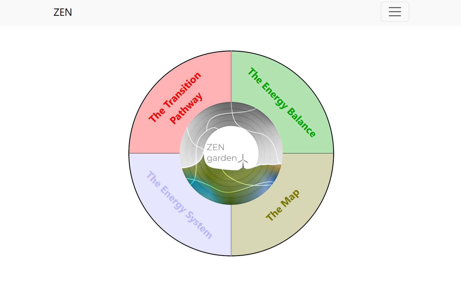
Fig. 1 Homepage of the ZEN-garden visualization platform.
Example Exercises
Use the ZEN-Garden visualization platform to identify the total the total capacity of natural gas boilers in 2023 in (a) Germany, (b) Switzerland, and (c) total.
To answer this question, select the following options on the visualization tool:
Click on “The Transition Pathway.”
Click on “Capacity.”
Select the following options when asked: Solution =
5_multiple_time_steps_per_year, Variable =capacity, Technology Type =conversion, Carrier =heat. These options tell the visualization platform to look at all conversion technology capacities in the output5_multiple_time_steps_per_yearfor technologies which either produce or consume heat.You can now hover your cursor over the shown diagram to identify the total capacity of natural gas boilers installed in the model. To get capacities for individual countries, you can select which countries you would like to look at in the menu called
Node.
Solution: CH = 31 GW, DE = 187 GW, Total = 218 GW
For Germany in 2023, what hour of the simulation has the highest electricity demand?
To answer this question, select the following options on the visualization tool:
Click on “The Energy Balance”.
Click “Nodal Energy Balance”.
Select the following options when asked: Solution =
5_multiple_time_steps_per_year, Year =2023, Node =Germany, Carrier =electricity. These options tell the visualization platform to display an hourly electricity balance for Germany in 2023.You can now hover your cursor over the hour which has the highest electricity demand. A pop-up bubble should then show the hour during which that demand value occurred and the demand value at that time.
Solution: Hour Number = 89, Demand = 60.267 GW
Tip
You can investigate precomputed results from past studies with the visualization suite by visiting the following link: https://zen-garden.ethz.ch/. These studies contain much richer outputs than the example. They are thus ideal for exploring the platform’s full visualization potential.
Results Object
Detailed ZEN-garden results are stored in the output folder of the data
directory. ZEN-garden provides functions and tools for easily loading,
extraction, processing, and aggregation of outputs. This tutorial describes
how to use the most basic functions from ZEN-garden results processing. All
code chunks in this section refer to Python code.
The easiest way to access the results values is to import raw data into an
object of the the Results class from the zen_garden package. To do this,
open a python editor (e.g. Pycharm, VSCode or Jupyter Notebook) and activate
the ZEN-garden environment. Then, load the results with the following code:
from zen_garden import Results
r = Results(path='<result_folder>')
The path <result_folder> is the path to the results folder of the dataset,
e.g., <data>/output/<dataset_name>.
The results class has many methods (i.e. functions) which can be used to access subsets of the results. The sections below describe some of the most important methods and how they can be used.
Read variables and parameters
The result codebase allows users to easily access all (1) sets of technologies
and nodes; (2) parameters of the original model ; (3) primal variable optimal
values; and (4) and dual variable optimal values. In the results code these four
elements are collectively referred to as components.
Step 1: Identify the name of the component
To filter the names by component type (<component_type> in {'parameter',
'variable', 'dual', 'sets'}) the following member function can be
used:
r.get_component_names(<component_type>)
For example, the following code produces a list of all variable names used in the model:
r.get_component_names('variable')
From the list of components names, select the component which your are interested in investigating. Descriptions of all components can be found in the in the documentation on sets, parameters, variables, and constraints.
Tip
Any component whose name starts with constraint_ refers to a dual
variable. Dual variables are not saved to the results by default. To view
dual variables, users therefore need to adjust the ZEN-garden
configurations, as described in configurations tutorial
Step II: Read component values
Once you have identified the name of the component you would like to investigate, several methods enable easy access to the component values. These are:
r.get_full_ts(<component_name>): Returns the full time series values of the component. In case of hourly-resolved data, the time series has a length of 8760 times the number of years simulated.r.get_total(<component_name>): Returns annual total values of the component. For components which are resolved hourly, all values within the same year are summed together.r.get_dual(<component_name>): Returns the dual values of the constraints.r.get_unit(<component_name>): Returns the units of the component.r.get_doc(<component_name>): Returns the documentation string of the component.
To access the annual capacity values of all technologies, for example, you can use the following code:
r.get_total('capacity')
This code returns a pandas multi-index DataFrame showing the capacity of all technologies in all years and all regions (see :ref:` image below <t_analyze.fig.capacity_results`>).
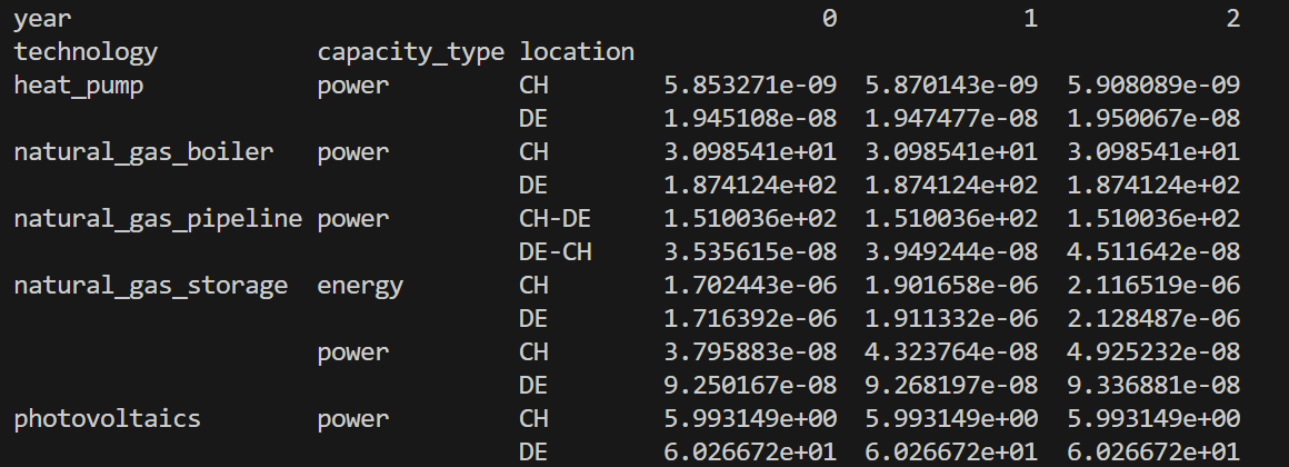
Fig. 2 Output of r.get_total('capacity').
Step III: Filter component values
The above functions (get_full_ts, get_total, get_dual, get_unit,
and get_doc) each allow optional input arguments for further narrowing the
results to values from a single scenario, year, or region. The optional input
arguments for these functions are:
year: A single optimization period for which the results should be returned (0, 1, 2, …). Note that this is not available forr.get_unit().scenario_name: A single scenario name for which the results should be returned. This is only relevant when using the scenario tool, as described in the scenarios tutorial.index: A slicing index for the results, i.e., a list of indices that of the dataframe for which results should be returned.
There are four ways to pass an index:
A single index, e.g.,
r.get_total('capacity', index="heat_pump"). This returns the capacity of heat pump for all other indices (e.g., nodes and years). Importantly, the index must correspond to the first index of the component.A list of indices, e.g.,
r.get_total('capacity', index=["heat_pump",
"photovoltaics"])
. This returns the capacity of heat pump and photovoltaics for all other indices. Importantly, the index must correspond to the first index of the component.A tuple of indices, e.g.,
r.get_total('capacity', index=("heat_pump", None,
["DE","CH"]))
. This returns the capacity of heat pump in the nodes DE and CH. The order of index levels matters. The value of a key can either be a single index, None, or a list of indices. In case of None, all indices of the corresponding level are returned.A dictionary, e.g.,
r.get_total('capacity', index={"node": ["DE", "CH"],
"technology": "heat_pump"})
. This returns the capacity of heat pump in the nodes DE and CH. The value of a key can either be a single index or a list of indices. The dictionary must contain the keys of the component. Since the key is passed, the order of the keys does not matter.
r.get_unit() has the additional argument convert_to_yearly_unit (default: False).
If set to True, the function converts the unit of the component to a yearly unit,
i.e., multiplying the unit string of components with an operational time step type with hour.
r.get_unit() can also be used to read the unit of the objective function with
r.get_unit('objective').
Note
The result class can only identify the components present in the result
files. Please refer to Solver on how to only save
selected parameters and variables. If the user wants to access a component
that was not saved, the user must add the component to the
selected_saved_parameters or selected_saved_variables in the
solver settings.
Example Exercises
Use the ZEN-Garden results code to identify the total the total capacity of natural gas boilers in 2023 in (a) Germany, (b) Switzerland, and (c) total to meet the heat demand.
To answer this question, the following code can be used:
from zen_garden import Results
r = Results(path='<result_folder>')
capacity_CH = r.get_total('capacity', index=("natural_gas_boiler", None, "CH"), year = 0).iloc[0,0]
capacity_DE = r.get_total('capacity', index=("natural_gas_boiler", None, "DE"), year = 0).iloc[0,0]
print(f"German Capacity: {capacity_DE}")
print(f"Swiss Capacity: {capacity_CH}")
print(f"Total Capacity: {capacity_DE + capacity_CH}")
Solution: CH = 31 GW, DE = 187 GW, Total = 218 GW
For Germany in 2023, what hour of the simulation has the highest electricity demand?
To answer this question, the following code can be used:
from zen_garden import Results
import numpy as np
r = Results(path='<result_folder>')
demand_DE = r.get_full_ts('demand', index=("electricity", "CH"), year=0)
hour = np.argmax(demand_DE)
max_demand = np.max(demand_DE)
print(f"Hour Number: {hour}")
print(f"Demand: {max_demand}")
Solution: Hour Number = 89, Demand = 60.267 GW
Comparing results
ZEN-garden provides methods to compare two different result objects. This can be helpful to understand why two results differ. Furthermore, it allows for a fast way to spot errors in the datasets. The most useful application is to compare the configuration (Configurations) of two datasets and the parameter values. Comparing variable values is often not very informative, as the results mostly differ in a large variety of variables.
Let’s assume you have the following two result objects:
from zen_garden import Results
r1 = Results(path='<result_folder_1>')
r2 = Results(path='<result_folder_2>')
Then you can compare the two result objects with the following code:
from zen_garden import compare_model_values, compare_configs
compare_parameters = compare_model_values([r1, r2], component_type = 'parameter')
compare_variables = compare_model_values([r1, r2], component_type = 'variable')
compare_config = compare_configs([r1, r2])
Per default, compare_model_values compares the total annual values of
components (Results Object). If the user wants to compare the
full time series, the optional argument compare_total=False can be passed
to the function. compare_model_values also accepts component_type =
"dual" and component_type = "sets". compare_configs compares the
configurations of the two datasets.