Tutorial 7: Scaling
What is scaling and when to use it?
Simply put, with scaling we aim at enhancing the numeric properties of a given optimization problem, such that solvers can solve it more efficiently and faster. It is generally recommended to include scaling, if the optimization problem at hand faces numerical issues or requires a long time to solve.
Scaling is done by transforming the coefficients of the decision variables in both constraints and objective function to a similar order of magnitude. In more mathematical terms, consider an optimization problem of the form:
Where \(x \in \mathbb{R}^n\) is the vector of decision variables, \(A \in \mathbb{R}^{m \times n}\) is the constraint matrix, \(b \in \mathbb{R}^m\) is the right-hand side vector and \(c \in \mathbb{R}^n\) is the cost vector. Note, that in ZEN-garden the constraints and optimization problem formulation can be generally of any form, however, for simpler notation we consider here the above form. If we now choose appropriate positive values for the column scaling vector \(s = [s_1, s_2, ..., s_n]\) and row scaling vector \(r = [r_1, r_2, ..., r_m]\), we can scale the optimization problem with the two diagonal matrices \(S = diag(s)\) and \(R = diag(r)\), such that the scaled optimization problem is:
If done successfully the scaled optimization problem has beneficial numeric properties such that it is less computational expensive to solve compared to the original formulation. Note that the objective value remains the same and that the problem’s solution is rescaled automatically within ZEN-garden so that also the decision variables are in the original scale.
Scaling Algorithms
In ZEN-garden we provide 3 different scaling algorithms, from which the row and column scaling vector entries are determined:
(Approximated) Geometric Mean (
"geom")Arithmetic Mean (
"arithm")Infinity Norm (
"infnorm")
The approximated geometric mean is the root of the product of the maximum and minimum absolute values of the respective row or column of the constraint matrix \(A\). The arithmetic mean is derived over all absolute values of the respective row or column of the constraint matrix \(A\). The infinity norm is the maximum absolute value of the respective row or column of the constraint matrix \(A\). For a more detailed explanation of each algorithm please see the paper from Elble and Sahinidis (2012).
Combination of Scaling Algorithms
While the scaling algorithms can be used individually, they can also be combined. In this case, over multiple iterations you can apply a sequence of different scaling algorithms. See How to use scaling in ZEN-garden? for more information.
Right-Hand Side Scaling
Furthermore, for all of the above mentioned algorithms, also the right-hand side vector \(b\) can be included in the scaling process. If included, the chosen algorithm determines the row scaling vector entry for a specific row \(i\) over all entries of that row in the constraint matrix \(A_{i*}\) while also considering the respective right-hand side entry \(b_i\).
How to use scaling in ZEN-garden?
As described in, Configurations in the Solver section, scaling can
be activated by adjusting the analysis.json file. The scaling configuration
can be chosen through the following three settings:
use_scaling: Boolean, whether scaling should be used or not.scaling_algorithm: List of strings, the scaling algorithms to be used. Possible entries are:"geom","arithm","infnorm". The length of the list determines the number of iterations.include_rhs: Boolean, whether the right-hand side vector should be included for determining the row scaling vector or not.
For example, the following configuration would use a combination of two iterations of the geometric mean scaling followed by one iteration of the infinity norm algorithm as well as taking into account the right-hand side vector:
"solver": {
  "use_scaling": true,
  "scaling_algorithm": ["geom", "geom","infnorm"],
  "scaling_include_rhs": true
}
The default configuration are three iterations of the geometric mean scaling algorithm with right-hand-side scaling.
Recommendations for using scaling
Here are some recommendations on what configuration to use and when and when not to use scaling. These rules were derived from the results of benchmarking the scaling procedure on different optimization problems as shown Results of benchmarking. Please note that these recommendations are general and are likely to not apply to all optimization problems. They rather serve as a starting configuration which then can be adjusted based on the problem at hand via for example trial and error.
Which algorithm to choose and how many iterations?
The benchmarking indicated a convergence of the numerical range of the scaled optimization problem mostly after the third iteration. Therefore, it is recommended to use at least three iterations of the scaling algorithm. The geometric mean scaling algorithm and the combination of geometric mean followed by infinity norm scaling showed the overall best performance across the considered optimization problems. Therefore, it is recommended to use one of the following configurations:
scaling_algorithm:["geom", "geom", "geom"]scaling_algorithm:["geom", "geom", "infnorm"]
When to include the right-hand side vector?
The benchmarking showed that including the right-hand side vector in the scaling
process leads to a better performance of the solver for almost all optimization
problems considered. Therefore, it is recommended to include the right-hand side
vector in the scaling process by setting scaling_include_rhs: True.
When not to use scaling?
If the optimization problem already has a good numerical range (which can be
checked with "solver": {"analyze_numerics": true}), scaling might not be
necessary. Also if the optimization problem already solves fast, the time
necessary for scaling the problem might outweigh the time savings from solving
the scaled optimization problem. As a rule of thumb, if the time to solve the
optimization problem is in similar order of magnitude as the time to scale the
problem, scaling should not be applied. The time necessary for scaling can be
checked in the output of the optimization problem, if scaling is applied.
How to deal with other complementary solver settings?
Some solvers might also have their own scaling algorithms or other algorithms to
improve the numerical properties of the optimization problem. In our
benchmarking, we examined the interaction of the respective functionalities of
Gurobi and scaling in ZEN-garden. Gurobi has the two options ScaleFlag and
NumericFocus that aim at improving numerical properties. The following
recommendations can be given based on the results of the benchmarking:
NumericFocusshould be set to its default value0.ScaleFlagshould be set to0(off) as the scaling in ZEN-garden already takes care of scaling the optimization problem and scaling the problem twice led on average to longer solving times. However, this varied across the optimization problems and therefore this again serves more as a default value to start with and should be tested for the specific problem at hand.
For similar functionalities in other solvers, it is recommended to test the interaction of the respective functionalities with the scaling in ZEN-garden via trial and error.
Results of benchmarking
The scaling functionality was benchmarked by running the following set of models with various scaling configurations:
Model |
Type |
#Variables |
#Constraints |
RHS range |
LHS range |
|---|---|---|---|---|---|
PI_small |
only electricity and heating sector, no strong year coupling through expansion constraints |
1092999 |
1636234 |
9 |
9 |
WES_nofe |
whole-energy system, year coupling through expansion constraints for each node individually (most complex case study) |
4191392 |
7039066 |
11 |
8 |
WES_nofe_PI |
whole-energy system, year coupling through expansion constraints for each node individually (most complex case study) |
11 |
8 |
||
WES_nofe_PC |
whole-energy system, year coupling through expansion constraints for each node individually (most complex case study) |
11 |
8 |
||
NoErr |
whole-energy system, year coupling through expansion constraints for all nodes together |
4196124 |
7017047 |
12 |
11 |
Snapshot |
single-year optimization |
1834197 |
1636205 |
7 |
8 |
Operation |
operational optimization |
4911453 |
1420119 |
9 |
8 |
Overall, for the purpose of benchmarking over all models a total number of 3250 runs were collected. The following sections will display the results of the benchmarking analysis and should provide insights about the effectiveness and functionality of the scaling algorithm.
Numerical Range vs. Number of Iterations
As argued in Recommendations for using scaling the numerical range showed
convergence in most cases after just three iterations. The following results of
running the scaling algorithms geometric mean (geom) and arithmetic mean
(arithm) for the model PI_small for different number of iterations,
portrays this result:
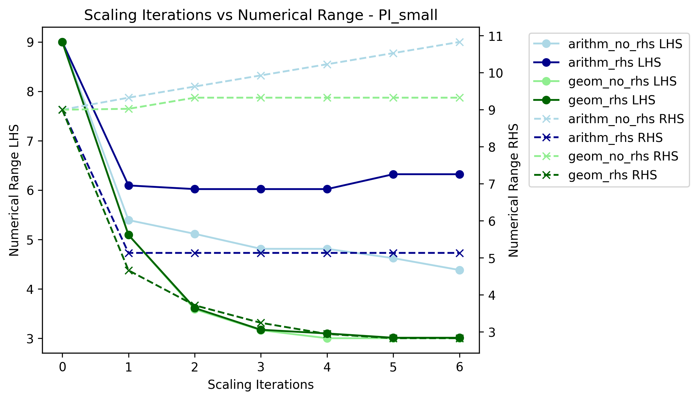
The dots indicate the left-hand side (LHS) range, which corresponds to the range of the A-matrix \(A\), whereas the crosses represent the numerical range of the right-hand side (RHS) vector \(b\). Light colors indicate the respective scaling configurations that exclude the right-hand side in the derivation of the row scaling vector.
From the plot we can observe:
convergence of the numerical range (of the LHS) is visible for both algorithms after three iterations
a trade-off between a lower LHS range and also decreasing the RHS range may exist, which is visible in case of arithmetic mean scaling
neglecting the RHS may lead to a significant increase in its numerical range, which is visible for both scaling algorithms (as shown in Regression Analysis this also leads on average to longer solving times)
Net-solving time comparison for multiple scaling configurations
The following plots show the net-solving time (solving time + scaling time) for
the models PI_small and NoErr. These models were chosen as they
represent very different results in terms of effectiveness of scaling. The model
PI_small showed mostly a significant decrease in net-solving time when
scaling was applied, whereas the model NoErr showed no significant effect of
scaling on the net-solving time or even worse an increase in solving-time.
Note, that the notation used for the ticks on the x-axis follows the pattern
<scaling_algorithm>_<number of iterations>_<include_rhs>. For example,
geom_3_rhs indicates the geometric mean scaling algorithm with three
iterations and including the right-hand side vector for deriving the row scaling
vector. A combination of geom and infnorm, where geometric mean scaling
is followed by infinity norm scaling, is indicated by geom_infnorm.
PI_small
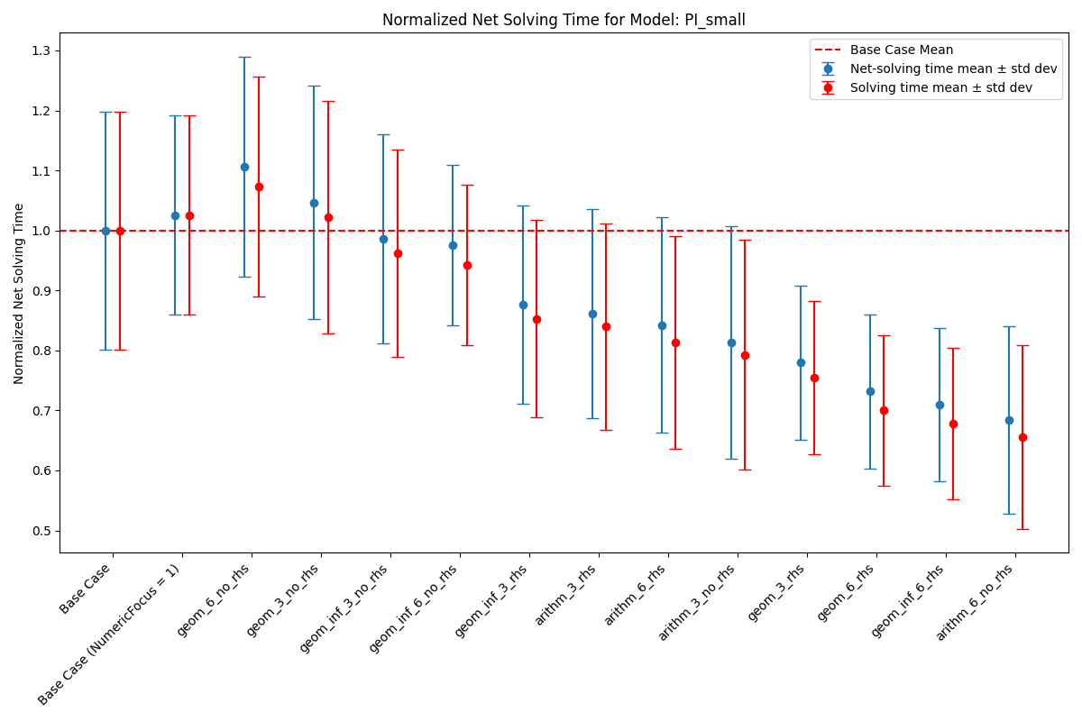
Note that the Base Case refers to a configuration where Gurobi scaling with
a NumericFocus of 0 is applied, but no scaling in ZEN-garden. Since for
this model all scaling configurations that use ZEN-garden are run with a fixed
NumericFocus of 1 (corresponding to low numeric focus), we also included
a Base Case configuration with a NumericFocus of 1 for comparison.
The red dotted line indicates the arithmetic mean of the net-solving time for
the base case configuration. Red dots represent the solving time without the
time spent on scaling the problem, whereas the blue dots represent the
net-solving time that includes both.
The plot shows:
a significant decrease in net-solving time for the model
PI_smallfor a majority of the considered algorithms when ZEN-garden scaling is appliedon average configurations that include the right-hand side vector for deriving the row scaling vector indicate a better performance
solving times are very inconsistent leading to large variances in the net-solving time for each scaling algorithm
scaling time only makes up a small fraction of the net-solving time
NoErr
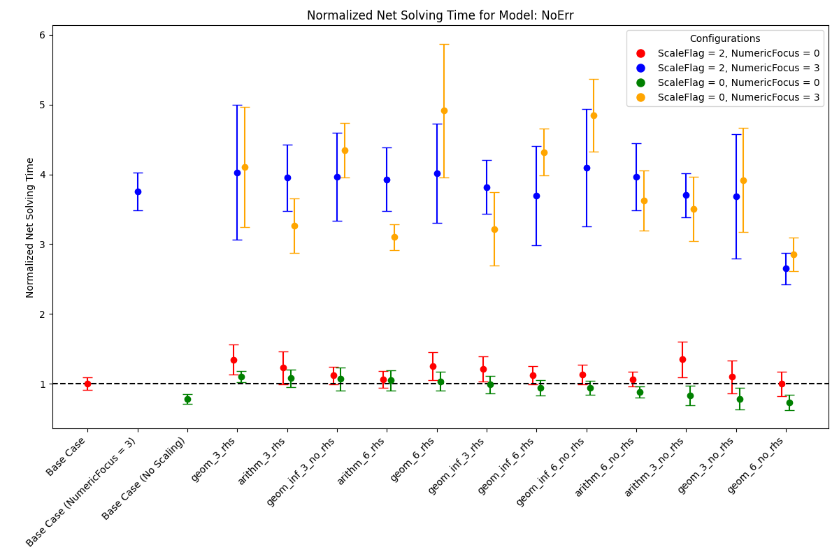
In the analysis of the model NoErr we set special focus on the interaction
and compatibility of ZEN-garden scaling with the numeric settings of Gurobi.
For this we included for each algorithm four configurations with different
combinations of ZEN-garden scaling and Gurobi’s ScaleFlag and
NumericFocus. A ScaleFlag of 2 indicates that Gurobi scaling is
turned on and thus double scaling (ZEN-garden and Gurobi) is applied. A
NumericFocus of 0 indicates an automatic numeric focus, whereas a
NumericFocus of 3 indicates high numeric focus. Again, the base cases
correspond to no ZEN-garden scaling.
From the plot we can derive:
a configuration where no scaling is applied (neither ZEN-garden nor Gurobi) can also lead to the best performance (as indicated by
Base Case (No Scaling))double scaling (ZEN-garden and Gurobi scaling) does not seem to be beneficial and rather increases the net-solving time
setting a high numeric focus increases the net-solving time significantly for all scaling configurations
only for a very few algorithms net-solving time is decreased when ZEN-garden scaling is applied and only for an automatic numeric focus and no Gurobi scaling
The two examples shown here, again indicate that deriving a general recommendation for the scaling configuration is difficult and that the performance of the scaling algorithm is highly dependent on the optimization problem at hand. Therefore, we recommended to test different scaling algorithms and configurations via trial and error.
Regression Analysis
Based on the collected data from the benchmarking runs for the models
PI_small, WES_nofe, WES_nofe_PI, and WES_nofe_PC, a regression
is run with the net-solving time (solving time + scaling time) as the dependent
variable. The explanatory variables are the models, the use_scaling boolean,
the include_rhs boolean, the NumericFcous (\(0\) or \(1\))
setting of Gurobi as well as an interaction term between ZEN-garden scaling and
Gurobi’s ScaleFlag. The results of the regression analysis are the
following:
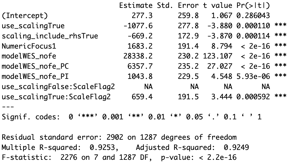
The key takeaways from the regression analysis are:
including ZEN-garden scaling decreases the net-solving time significantly
including the RHS for the derivation of the row scaling vectors decreases the net-solving time significantly
choosing a low
NumericFocusinstead of the automatic one, increases the net-solving time significantlydouble scaling, which means scaling both in ZEN-garden as well as within the solver (here Gurobi), seems to increase the net-solving time significantly
Please note, that these results can not be generalized. They only represent the average effect observed for the models considered here and might vary from case to case.