Dataset Examples

ZEN-garden provides a number of small datasets to demonstrate the functionalities of ZEN-garden and to understand the data structure. If you cloned the ZEN-garden repository, the datasets are in the docs/dataset_examples directory. Otherwise, download any of them with zen-example --dataset="<name>" (see Using dataset examples).

The following datasets are available:

• 1_base_case

• 2_multi_year_optimization

• 3_reduced_import_availability

• 4_multiple_time_steps_per_year

• 5_reduced_import_availability_yearly

• 6_time_series_aggregation

• 7_yearly_variation

• 8_myopic_foresight

• 9_brown_field

• 10_multi_scenario

• 11_multiple_in_output_carriers_conversion

• 12_yearly_interpolation

• 13_retrofitting_and_fuel_substitution

• 14_unit_consistency_expected_error

All datasets build upon 1_base_case and extend it with additional features. Each description below highlights the difference to the previous dataset.

1_base_case

The base case includes a simple energy system consisting of two nodes: Switzerland (CH) and Germany (DE). Although more nodes are defined in the set_nodes.csv file, only CH and DE are selected in system.yaml. A single year optimization fulfils the heat and electricity demands in both nodes. To fulfil the demands, the energy system can install and use the following technologies:

Table 9 Technologies in the base case

Name	Technology type	Description
Natural gas boiler	Conversion	Converts natural gas to heat
Photovoltaics	Conversion	Generates electricity
Natural gas storage	Storage	Stores natural gas
Natural gas pipeline	Transport	Transports natural gas between nodes

Resulting from the technologies, the model requires the energy carriers heat, electricity, and natural gas. As only natural gas boilers can produce heat in this example, the optimal solution builds the boilers in both nodes to fulfil the heat demand. In both nodes, photovoltaic systems generate the required electricity. Natural gas pipeline and storage are not installed as the natural gas can be imported in both nodes without limits.

2_multi_year_optimization

The model builds upon the base case by extending the optimization over multiple years. The parameter optimized_years in the system.yaml file defines the number of years to optimize. Additionally, the optimization only runs for every second year, thus, aggregating two years in each optimized year. This setting can be controlled with the interval_between_years parameter in the system.yaml file. The heat demand in both nodes is variable over the years and the optimization model must fulfil them in all years. The adjusted heat demand is specified in the demand.csv file of the heat folder.

3_reduced_import_availability

The example is identical to 2_multi_year_optimization, but with reduced import availability of natural gas in DE (see the file availability_import.csv). The reduced import availability forces the model to install natural gas pipelines to transport the missing natural gas from CH to DE. Additionally in this model, natural gas pipeline capital expenditures consist of two parts, which are independent: distance dependent costs (capex_per_distance_transport) and capacity dependent costs (capex_specific_transport). These costs are specified independently from each other in the attributes.yaml file. Note that the units of capex_per_distance_transport need to be specified as costs per distance without taking into account the capacity. The distance dependent costs depend on a binary decision whether the connection is installed or not, while the capacity dependent costs are linearly dependent on the installed capacity. Consequently, the model is a mixed integer linear program. This method for calculating the costs of transport modes needs to be activated in the system.yaml file by setting the parameter double_capex_transport to true.

4_multiple_time_steps_per_year

Now the model includes time steps within a year and optimizes the operation of the energy system. In the system.yaml file the parameters aggregated_time_steps_per_year and unaggregated_time_steps_per_year are set to 96. This equals looking at the first 96 hours of the year. In order to include variation between the time steps, the electricity and heat demands are hourly resolved in the demand.csv file.

5_reduced_import_availability_yearly

With the file availability_import_yearly.csv the import availability of natural gas in CH is step-wise reduced for each year. In contrast to the availability_import.csv file, the availability_import_yearly.csv file specifies the limit for the entire year and not for individual time steps. As a consequence of the import restrictions, the solution contains natural gas storage and pipelines to store natural gas for the years with a smaller import limit.

6_time_series_aggregation

Now the time series aggregation is switched on in the system.yaml file by setting the parameter conduct_time_series_aggregation to true. Additionally, the parameter aggregated_time_steps_per_year needs to be smaller than the unaggregated_time_steps_per_year. In this example, 96 time steps are aggregated to 10 representative time steps. For illustration purposes, the availability_import_yearly.csv file of natural gas is structured differently from the previous examples:

Table 10 Yearly import availability of natural gas in CH

node	2023	2024	2025
CH	inf	80	40

The years are now set as the columns of the file and the nodes as the rows. Both structures are supported in ZEN-garden and depending on the input data, one might be easier to handle than the other.

7_yearly_variation

In addition to the variation within a year, ZEN-garden’s input data can also handle variation between years. The yearly variation multiplies a parameter with a constant factor for the entire year. Consequently, the shape of the input data is the same for each year, but the scale is different. In this example, the price of natural gas and the electricity demand are varied between the years. For natural gas, the file price_import_yearly_variation.csv contains the factor to for each year. The factors for the electricity demand are stored in the file demand_yearly_variation.csv. For example, the factor for electricity demand in DE in year 2029 is 1.2. The electricity demand of each hour is, therefore, multiplied with the factor 1.2 for the entire year 2029 leading to a proportional increase of the electricity demand. Additionally, the example optimizes the full year instead of only the first 96 hours. The parameter unaggregated_time_steps_per_year is set to 8760 in the system.yaml file. However, the time series aggregation is still active and the optimization uses 10 representative time steps for the entire year.

8_myopic_foresight

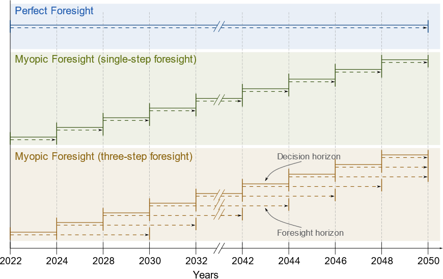
All the previous datasets are optimized using so-called perfect foresight, i.e., all years are optimized at once with the assumption that all the future parameter data are known at the time the optimization is conducted. In this example, however, myopic foresight is demonstrated, where the knowledge of future parameter data, the foresight horizon, is limited. To activate this feature, the parameter use_rolling_horizon in the system.yaml file is set to true. Simultaneously, the years_in_rolling_horizon parameter needs to be specified to set the length of the foresight horizon. In this example, the foresight horizon is set to 1.

The difference between perfect and myopic foresight is illustrated in the following figure, where the lengths of the decision horizon and the foresight horizon are visualized:

9_brown_field

Up to this model, all examples have assumed so-called green field capacity expansion. The assumption is that all capacities are newly built and no capacities are existing on nodes or edges, i.e., the whole system is built from scratch. In this model, the brown field capacity expansion is introduced. Brown field capacity expansion means that some capacities already exist and have to be considered in the optimization. ZEN-garden supports existing capacities that are built in the past, i.e., can be used immediately and have a reduced lifetime left. Additionally, capacities that will be built in the future, i.e. within the optimization horizon, can be considered. For example, this may cover installations for which the decision to build them has already been made, but the construction has not yet started. The model 9_brown_field builds upon the example 7_yearly_variation, i.e., with perfect foresight optimization. For photovoltaic systems, the file capacity_existing.csv is added which specifies the capacities that exist in the nodes and the year in which they were or will be built.

10_multi_scenario

The model 10_multi_scenario showcases the scenario analysis feature of ZEN-garden. The parameter conduct_scenario_analysis in the system.yaml file is set to true and a new file, scenarios.yaml, is added to the dataset. The file scenarios.yaml contains the different scenarios that are considered in the optimization. In the example, all supported ways of manipulating the input data are demonstrated. Additional files are added to the dataset which are used by the different scenarios: different carbon prices and a new attributes file for electricity. The files which are to be used by the scenario analysis must have an additional ending in the file name to distinguish them from the standard input data files. The ending is specified in the scenarios.yaml file. For example, the alternative attributes file for electricity is named attributes_low_carbon.yaml.

11_multiple_in_output_carriers_conversion

This model introduces conversion technologies which work with more than one in- or output carrier. For this purpose, the model from example 7_yearly_variation is extended with a combined heat and power (CHP) technology. The CHP technology replaces the natural gas boiler and works with natural gas and biogas as input carriers. The carrier biogas is newly introduced as well. The output carriers of the CHP plant are heat and electricity. The ratio in which the CHP plant uses natural gas/biogas and produces heat/electricity is specified with the conversion_factor parameter of the CHP plant. The respective parameter in the attributes.yaml file of the CHP plant is specified as:

conversion_factor:
  heat:
    default_value: 1.257
    unit: GWh/GWh
  natural_gas:
    default_value: 1.427
    unit: GWh/GWh
  bio_gas:
    default_value: 1.427
    unit: GWh/GWh

12_yearly_interpolation

This example showcases how missing values in input data can be interpolated and how the interpolation can be switched off. Compared to the previous example, an annual limit of carbon emissions is introduced (file carbon_emissions_annual_limit.csv). Each of the parameters carbon_emissions_annual_limit and price_carbon_emissions have yearly values missing. Per default, ZEN-garden interpolates the missing values linearly between the two closest known values. If this behaviour is not wanted, parameter names can be added to the file parameters_interpolation_off.yaml inside the energy_system folder. For the parameter names in this file, the interpolation of missing values is switched off. In this case, the default value from the attributes.yaml file is used for the missing values.

13_retrofitting_and_fuel_substitution

In this example, the concept of retrofit technologies is introduced. Retrofit technologies are technologies that can be added to existing technologies to change their input or output carriers. By changing the input carrier of a technology, the model can substitute the fuel originally used by the technology with another fuel. In this example, the CHP plant can be retrofitted to use e-fuel instead of natural gas. This is done with the newly added technology e_fuel_production which takes electricity as input and produces natural gas. Another retrofit technology is the carbon_capture technology which can be added to the CHP plant to capture the carbon emissions. It requires electricity as input and produces carbon which is then stored permanently with another added technology: carbon_storage.

Since the retrofit technology can only be added to a specific conversion technology, it requires an additional parameter in the attributes.yaml file:

retrofit_flow_coupling_factor:
  base_technology: CHP_plant
  default_value: 0.18
  unit: kilotons/GWh

The retrofit_flow_coupling_factor specifies to which technology the retrofit technology can be added and the coupling factor between the retrofit and the base technology. The retrofit technologies belong to a new technology set: set_retrofitting_technologies, which must be specified in the system.yaml file. The set retrofitting technologies is a child of the conversion technologies and, therefore, the folder for carbon_capture and e_fuel_production must be places inside the folder set_conversion_technologies. Since carbon_capture and carbon_storage require carbon as an input/output carrier, carbon is included in the dataset.

14_unit_consistency_expected_error

The example should illustrate the ZEN-garden response in case the input data is faulty. Specifically, ZEN-garden checks whether the units of the input data are consistent between technologies and carriers. In the example, several units of the carrier natural_gas and the technology natural_gas_pipeline are changed from an energy-based unit (GWh) to a mass-based unit (tons). When running the example, ZEN-garden will raise an error due to the unit inconsistency.